ជំពូក៥ : ដេទែរមីណង់

October 2nd, 2020

From Wikipedia:

The volume of this parallelepiped is the absolute value of the determinant of the matrix formed by the columns constructed from the vectors: $\vec r_1, \vec r_2$, and $\vec r_3$.

ក្នុងគណិតវិទ្យា determinant is a scalar value that is a function of the entries of a square matrix. It allows characterizing some properties of the matrix and the linear map represented by the matrix. In particular, the determinant is nonzero if and only if the matrix is invertible and the linear map represented by the matrix is an isomorphism. The determinant of a product of matrices is the product of their determinants (the preceding property is a corollary of this one)

The determinant of $A$ is denoted by $\det(A)$, or it can be denoted directly in terms of the matrix entries by writing enclosing bars instead of brackets: \[ |A| = \begin{vmatrix}a_{11}&a_{12}&\cdots &a_{1n}\\a_{21}&a_{22}&\cdots &a_{2n}\\\vdots &\vdots &\ddots &\vdots \\a_{n1}&a_{n2}&\cdots &a_{nn}\end{vmatrix} \] There are various equivalent ways to define the determinant of a square matrix A, i.e. one with the same number of rows and columns: the determinant can be defined via the Leibniz formula, an explicit formula involving sums of products of certain entries of the matrix. The determinant can also be characterized as the unique function depending on the entries of the matrix satisfying certain properties. This approach can also be used to compute determinants by simplifying the matrices in question.

Outcomes

គណនាដេទែរមីណង់របស់ម៉ាទ្រីសការេ ដោយប្រើ ពន្លាតឡាផ្លាស់ (Laplace Expansion) ឬ ពន្លាតកូហ្វាក់ទើរ (Cofactor Expansion) ឬប្រើ ប្រមាណវិធីជួរដេក (row operations)។
Demonstrate the effects that row operations have on determinants.
Verify the following:
1. The determinant of a product of matrices is the product of the determinants.
2. The determinant of a matrix is equal to the determinant of its transpose.

Basic Techniques

Let $A$ be an $n\times n$ matrix, that is, a square matrix. The determinant of $A$, denoted by $\det(A)$ or $|A|$ is a very important number which we will explore throughout this section.

If $A$ is a 2$\times 2$ matrix, the determinant is given by the following formula.

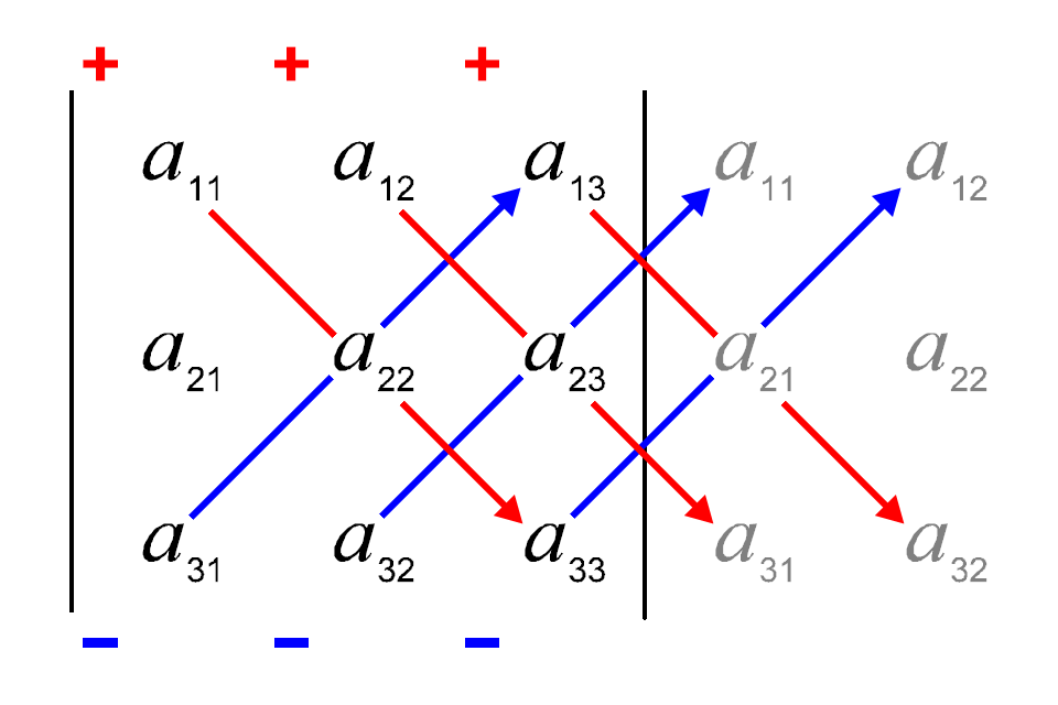
(Sarrus's Rule for $2\times 2$ and $3\times 3$-Matrices)

By Sarrus' rule (1), the determinant of $2\times 2$ and $3\times 3$ matrices are defined as following:

Consider a $2\times 2$ matrix \[A=\left[ \begin{array}{rr} a & b \\ c & d \end{array} \right] \] Then, the determinant of $A$ is defined by \[\det \left( A\right) = ad-cb\nonumber \]
And the determinant of a $3\times 3$ matrix $$ A=\begin{bmatrix}a_{11}&a_{12}&a_{13}\\a_{21}&a_{22}&a_{23}\\a_{31}&a_{32}&a_{33}\end{bmatrix}$$ can be computed by the following scheme \begin{eqnarray*} \det(A) &=& \begin{vmatrix}a_{11}&a_{12}&a_{13}\\a_{21}&a_{22}&a_{23}\\a_{31}&a_{32}&a_{33}\end{vmatrix}\\ &=& a_{11}a_{22}a_{33}+a_{12}a_{23}a_{31}+a_{13}a_{21}a_{32}\\ && \qquad \qquad -\; a_{31}a_{22}a_{13}-a_{32}a_{23}a_{11}-a_{33}a_{21}a_{12} \end{eqnarray*}

^{1. [The Rule of Sarrus is a mnemonic device for computing the determinant of a $ 3\times 3$ matrix named after the French mathematician Pierre Frédéric Sarrus (invented 1833).]↩}

Sarrush Rule

(Example A Two by Two Determinant )

Find $\det\left(A\right)$ for the matrix $A = \left[ \begin{array}{rr} 2 & 4 \\ -1 & 6 \end{array} \right] .$

Show solution

The $2 \times 2$ determinant can be used to find the determinant of larger matrices. We will now explore how to find the determinant of a $3 \times 3$ matrix, using several tools including the $2 \times 2$ determinant.

We begin with the following definition.

(The $ij^{th}$ Minor of a Matrix)

Let $A$ be a $3\times 3$ matrix. The $ij^{th}$ minor of $A$, denoted as $\minor\left( A\right) _{ij},$ is the determinant of the $2\times 2$ matrix which results from deleting the $i^{th}$ row and the $j^{th}$ column of $A$.

In general, if $A$ is an $n\times n$ matrix, then the $ij^{th}$ minor of $A$ is the determinant of the $n-1 \times n-1$ matrix which results from deleting the $i^{th}$ row and the $j^{th}$ column of $A$.

Hence, there is a minor associated with each entry of $A$. Consider the following example which demonstrates this definition.

(Finding Minors of a Matrix )

Let \[A = \left[ \begin{array}{rrr} 1 & 2 & 3 \\ 4 & 3 & 2 \\ 3 & 2 & 1 \end{array} \right] \] Find $\minor\left( A\right) _{12}$ and $\minor\left( A\right) _{23}$.

Show solution

(The $ij^{th}$ Cofactor of a Matrix)

Suppose $A$ is an $n\times n$ matrix. The $ij^{th}$ cofactor, denoted by $\mathrm{cof}\left( A\right) _{ij}$ is defined to be \[\cof\left( A\right) _{ij} = \left( -1\right) ^{i+j} \cdot \minor\left(A\right)_{ij} \] We denote as following:

$\cof (A) = \Big( \cof(A)_{ij} \Big)_{n\times n}$ ហៅថា ម៉ាទ្រីសកូហ្វាក់ទ័រ
$\mathbf{adj}(A) = \Big( \cof(A)_{ij} \Big)_{n\times n}^T$ ហៅថា ម៉ាទ្រីស adjoint បានមកពីត្រង់ស្ប៉ូ របស់ម៉ាទ្រីសកូហ្វាក់ទ័រ។

ចំណាំ : It is also convenient to refer to the cofactor of an entry of a matrix as follows. If $a_{ij}$ is the $ij^{th}$ entry of the matrix, then its cofactor is just $\cof\left( A\right) _{ij}$, or simply $A_{ij}$ or $c_{ij}$.

(Finding Cofactors of a Matrix)

Consider the matrix \[A=\left[ \begin{array}{rrr} 1 & 2 & 3 \\ 4 & 3 & 2 \\ 3 & 2 & 1 \end{array} \right]\nonumber \] Find $\cof\left( A\right) _{12}$ and $\cof\left( A\right) _{23}$.

Show solution

(The Determinant of a Three By Three Matrix)

Let $A$ be a $3\times 3$ matrix. Then, $\det \left(A\right)$ is calculated by picking a row (or column) and taking the product of each entry in that row (column) with its cofactor and adding these products together.

This process when applied to the $i^{th}$ row (column) is known as expanding along the $i^{th}$ row (column) as is given by \[\det \left(A\right) = a_{i1}\cdot\cof(A)_{i1} + a_{i2}\cdot\cof(A)_{i2} + a_{i3}\cdot\cof(A)_{i3}\nonumber \]

NOTE: When calculating the determinant, you can choose to expand any row or any column. Regardless of your choice, you will always get the same number which is the determinant of the matrix $A.$ This method of evaluating a determinant by expanding along a row or a column is called Laplace Expansion or Cofactor Expansion.

(Finding the Determinant of a Three by Three Matrix )

Let \[A=\left[ \begin{array}{rrr} 1 & 2 & 3 \\ 4 & 3 & 2 \\ 3 & 2 & 1 \end{array} \right]\nonumber \] Find $\det\left(A\right)$ using the method of Laplace Expansion.

Show solution

First, we will calculate $\det \left(A\right)$ by expanding along the first column. Using Definition $\PageIndex{4}$, we take the $1$ in the first column and multiply it by its cofactor, \[1 \left( -1\right) ^{1+1}\left| \begin{array}{rr} 3 & 2 \\ 2 & 1 \end{array} \right| = (1)(1)(-1) = -1\nonumber \] Similarly, we take the $4$ in the first column and multiply it by its cofactor, as well as with the $3$ in the first column. Finally, we add these numbers together, as given in the following equation. \[\det \left(A\right) = 1 \overset{ \cof\left( A\right) _{11}}{\overbrace{\left( -1\right) ^{1+1}\left| \begin{array}{rr} 3 & 2 \\ 2 & 1 \end{array} \right| }}+4 \overset{\cof\left( A\right) _{21}}{\overbrace{\left( -1\right) ^{2+1}\left| \begin{array}{rr} 2 & 3 \\ 2 & 1 \end{array} \right| }}+3 \overset{\cof\left( A\right) _{31}}{\overbrace{\left( -1\right) ^{3+1}\left| \begin{array}{rr} 2 & 3 \\ 3 & 2 \end{array} \right| }} \] Calculating each of these, we obtain \[\det \left(A\right) = 1 \left(1\right)\left(-1\right) + 4 \left(-1\right)\left(-4\right) + 3 \left(1\right)\left(-5\right) = -1 + 16 + -15 = 0 \] Hence, $\det\left(A\right) = 0$.

As mentioned in Definition $\PageIndex{4}$, we can choose to expand along any row or column. Let’s try now by expanding along the second row. Here, we take the $4$ in the second row and multiply it to its cofactor, then add this to the $3$ in the second row multiplied by its cofactor, and the $2$ in the second row multiplied by its cofactor. The calculation is as follows. \[ \det \left(A\right) = 4 \overset{\cof\left( A\right) _{21}}{\overbrace{\left( -1\right) ^{2+1}\left| \begin{array}{rr} 2 & 3 \\ 2 & 1 \end{array} \right| }}+3 \overset{\cof\left( A\right) _{22}}{\overbrace{\left( -1\right) ^{2+2}\left| \begin{array}{rr} 1 & 3 \\ 3 & 1 \end{array} \right| }}+2 \overset{\cof\left( A\right) _{23}}{\overbrace{\left( -1\right) ^{2+3}\left| \begin{array}{rr} 1 & 2 \\ 3 & 2 \end{array} \right| }} \] Calculating each of these products, we obtain \[\det \left(A\right) = 4\left(-1\right)\left(-2\right) + 3\left(1\right)\left(-8\right) + 2 \left(-1\right)\left(-4\right) = 0 \] You can see that for both methods, we obtained $\det \left(A\right) = 0$.

As mentioned above, we will always come up with the same value for $\det \left(A\right)$ regardless of the row or column we choose to expand along. You should try to compute the above determinant by expanding along other rows and columns. This is a good way to check your work, because you should come up with the same number each time! We present this idea formally in the following theorem.

Theorem 1. : (The Determinant is Well Defined)

Expanding the $n\times n$ matrix along any row or column always gives the same answer, which is the determinant, meaning that

\begin{eqnarray*} \begin{vmatrix} a_{11} & a_{12} & \cdots & a_{1n} \\ a_{21} & a_{22} & \cdots & a_{2n}\\ \vdots & \vdots & \ddots & \vdots \\ a_{n1} & a_{n2} & \cdots &a_{nn} \end{vmatrix} &= &\sum_{k=1}^{n} a_{ik} \cdot \cof(A)_{ik}, \quad (\text{by row } i\text{-th}, i=1,\ldots,n) \\ &= &\sum_{k=1}^{n} a_{kj} \cdot \cof(A)_{kj}, \quad (\text{by column } j\text{-th}, j=1,\ldots,n) \end{eqnarray*}

For example, the $ij^{th}$ minor of a $4 \times 4$ matrix is the determinant of the $3 \times 3$ matrix you obtain when you delete the $i^{th}$ row and the $j^{th}$ column. Just as with the $3 \times 3$ determinant, we can compute the determinant of a $4 \times 4$ matrix by Laplace Expansion, along any row or column Consider the following example.

(Determinant of a Four by Four Matrix)

Find $\det \left( A\right)$ where \[A=\left[ \begin{array}{rrrr} 1 & 2 & 3 & 4 \\ 5 & 4 & 2 & 3 \\ 1 & 3 & 4 & 5 \\ 3 & 4 & 3 & 2 \end{array} \right] \]

Show solution

The following provides a formal definition for the determinant of an $n \times n$ matrix. You may wish to take a moment and consider the above definitions for $2 \times 2$ and $3 \times 3$ determinants in context of this definition.

(The Determinant of an $n\times n$ Matrix)

Let $A$ be an $n\times n$ matrix where $n\geq 2$ and suppose the determinant of an $\left( n-1\right) \times \left( n-1\right)$ has been defined. Then \[\det \left( A\right) =\sum_{j=1}^{n}a_{ij}\cdot\cof\left( A\right) _{ij}=\sum_{i=1}^{n}a_{ij}\cdot\cof\left( A\right) _{ij}\nonumber \] The first formula consists of expanding the determinant along the $i^{th}$ row and the second expands the determinant along the $j^{th}$ column.

The Determinant of a Triangular Matrix

There is a certain type of matrix for which finding the determinant is a very simple procedure. Consider the following definition.

(Triangular Matrices)

A matrix $A$ is upper triangular if $a_{ij}=0$ whenever $i\gt j$. Thus the entries of such a matrix below the main diagonal equal $0$, as shown. Here, $\ast$ refers to any nonzero number. \[ \left[ \begin{array}{cccc} \ast & \ast & \cdots & \ast \\ 0 & \ast & \cdots & \vdots \\ \vdots & \vdots & \ddots & \ast \\ 0 & \cdots & 0 & \ast \end{array} \right]\nonumber \] A lower triangular matrix is defined similarly as a matrix for which all entries above the main diagonal are equal to zero.

Theorem 2: (Determinant of a Triangular Matrix)

Let $A$ be an upper or lower triangular matrix. Then $\det \left( A\right)$ is obtained by taking the product of the entries on the main diagonal.

The verification of this Theorem can be done by computing the determinant using Laplace Expansion along the first row or column.

(Determinant of a Triangular Matrix)

Let \[A=\left[ \begin{array}{rrrr} 1 & 2 & 3 & 77 \\ 0 & 2 & 6 & 7 \\ 0 & 0 & 3 & 33.7 \\ 0 & 0 & 0 & -1 \end{array} \right]\nonumber \] Find $\det \left( A\right) .$

Show solution

លក្ខណៈរបស់ដេទែរមីណង់

The determinant is an important notion in linear algebra.

(Basic definition)

Let $A(n\times n) = (a_{ij})$, the determinant is defined by the sum \begin{align*} \det(A) & = \sum_{\sigma \in S_n} \text{sign} (\sigma) a_{1\sigma(1)} a_{2\sigma(2)} \dotsc a_{n\sigma(n)} \\ & = \sum_{\sigma \in S_n} \text{sign}(\sigma) \prod_{i=1}^n a_{i\sigma(i)} \end{align*} where $S_n$ is the set of all permutations on the set $\{ 1, \dotsc, n\}$, and $\text{sign}(\sigma)$ is the parity of the permutation $\sigma$.

Simpler Definition: where $m_i$ is the $(n-1)\times(n-1)$ matrix formed by removing the $1$st row and $i$th column from $a$: \begin{eqnarray*} m_i &=& \begin{pmatrix} \blacksquare & \blacksquare & ... & \blacksquare & \blacksquare & \blacksquare & ... & \blacksquare & \blacksquare\\ a_{21} & a_{22} & ... & a_{2,i-1} & \blacksquare & a_{2,i+1} & ... & a_{2,n-1} & a_{2n}\\ a_{31} & a_{32} & ... & a_{3,i-1} & \blacksquare & a_{3,i+1} & ... & a_{3,n-1} & a_{3n}\\ &&&&\vdots&&&&\\ a_{n1} & a_{n2} & ... & a_{n,i-1} & \blacksquare & a_{n,i+1} & ... & a_{n,n-1} & a_{nn} \end{pmatrix}\\ & =& \begin{pmatrix} a_{21} & ... & a_{2,i-1} & a_{2,i+1} & ... & a_{2n}\\ a_{31} & ... & a_{3,i-1} & a_{3,i+1} & ... & a_{3n}\\ &&\vdots&\vdots&&&\\ a_{n1} & ... & a_{n,i-1} & a_{n,i+1} & ... & a_{nn} \end{pmatrix} \end{eqnarray*}

There are many important properties of determinants. Since many of these properties involve the row operations discussed in Chapter 1, we recall that definition now.

(Row Operations)

ប្រមាណវិធីជួរដេក (row operations) អនុវត្តទៅលើម៉ាទ្រីសមួយ ត្រូវបានកំណត់ដូចខាងក្រោម៖

Switch two rows $(R_i \longleftrightarrow R_j)$
Multiply a row by a nonzero number $(\lambda\cdot R_i^{\text{old}} \longrightarrow R_i^{\text{new}})$
Replace a row by a multiple of another row added to itself $(R_i^{\text{old}}+\lambda\cdot R_j^{\text{old}} \longrightarrow R_i^{\text{new}})$

We will now consider the effect of row operations on the determinant of a matrix. In future sections, we will see that using the following properties can greatly assist in finding determinants. This section will use the theorems as motivation to provide various examples of the usefulness of the properties.

Properties I: (the effect of row operations)

Switching Rows: យកម៉ាទ្រីស $A$ មានលំដាប់ $n\times n$ និងយក $B$ ជាម៉ាទ្រីសដែលបានមកពីការប្ដូរជួរដេកពីររបស់ម៉ាទ្រីស $ A$ ។ ដូច្នេះ គេបាន $$\det(B)=-\det(A)$$
Multiplying a Row by a Scalar: បើម៉ាទ្រីស $A$ មានលំដាប់ $n\times n$ និង $B$ ជាម៉ាទ្រីសដែលបានមក ដោយគុណជួរដេកណាមួយរបស់់ម៉ាទ្រីស $A$ ជាមួយនឹង ស្កាលែរ $k\neq 0$ ។ ដូច្នេះ គេបាន $$\det(B)=k\cdot\det(A)$$
Scalar Multiplication: យក $A$ និង $B$ ជាម៉ាទ្រីសលំដាប់ $n \times n$ និងកំណត់ $k$ ជាស្កាលែរមួយ ដែល $B = k\cdot A$ ។ ដូច្នេះ គេបាន \[\det(B) = k^n\cdot \det(A)\]
Adding a Multiple of a Row to Another Row: Let $A$ be an $n\times n$ matrix and let $B$ be a matrix which results from adding a multiple of a row to another row. Then \[\det \left( A\right) =\det \left( B \right)\]

សម្គាល់: We can carry out the same operations with columns, rather than rows. The three operations outlined in Definition $\PageIndex{1}$ can be done with columns instead of rows. In this case, in Theorems $\PageIndex{1}$, $\PageIndex{2}$, and $\PageIndex{4}$ you can replace the word, "row" with the word "column".

There are several other major properties of determinants which do not involve row (or column) operations. The first is the determinant of a product of matrices.

Properties II: (major properties of determinants)

Determinant of a Product: Let $A$ and $B$ be two $n\times n$ matrices. Then \[\det \left( AB\right) =\det \left( A\right) \det \left( B\right)\nonumber \]
Determinant of the Transpose: Let $A$ be a matrix where $A^T$ is the transpose of $A$. Then, \[\det\left(A^T\right) = \det \left( A \right)\nonumber \]
Determinant of the Inverse: Let $A$ be an $n \times n$ matrix. Then $A$ is invertible if and only if $\det(A) \neq 0$. If this is true, it follows that \[\det(A^{-1}) = \frac{1}{\det(A)}\nonumber \]

Properties of Determinants: Some Important Proofs

We will see some important proofs on determinants and cofactors. First we recall the definition of a determinant.

If $A=\left[ a_{ij} \right]$ is an $n\times n$ matrix, then $\det A$ is defined by computing the expansion along the first row: \begin{equation} \label{E1} \det(A) =\sum_{i=1}^n a_{1,i} \cdot \cof(A)_{1,i} \end{equation} If $n=1$ then $\det(A) =a_{1,1}$.

The following example is straightforward and strongly recommended as a means for getting used to definitions.

(Elementary Matrices - ម៉ាទ្រីសបឋម)

Let $E_{ij}$ be the elementary matrix obtained by interchanging $i$th and $j$th rows of $I$. Then $\det(E_{ij})=-1$.
Let $E_{ik}$ be the elementary matrix obtained by multiplying the $i$th row of $I$ by $k$. Then $\det(E_{ik})=k$.
Let $E_{ijk}$ be the elementary matrix obtained by multiplying $i$th row of $I$ by $k$ and adding it to its $j$th row. Then $\det(E_{ijk})=1$.
If $C$ and $B$ are such that $CB$ is defined and the $i$th row of $C$ consists of zeros, then the $i$th row of $CB$ consists of zeros.
If $E$ is an elementary matrix, then $\det(E)=\det(E^T)$.

Show solution

Many of the proofs in section use the Principle of Mathematical Induction. First we check that the assertion is true for $n=2$ (the case $n=1$ is either completely trivial or meaningless).

Next, we assume that the assertion is true for $n-1$ (where $n\geq 3$) and prove it for $n$. Once this is accomplished, by the Principle of Mathematical Induction we can conclude that the statement is true for all $n\times n$ matrices for every $n\geq 2$.

If $A$ is an $n\times n$ matrix and $1\leq j \leq n$, then the matrix obtained by removing $1$st column and $j$th row from $A$ is an $n-1\times n-1$ matrix (we shall denote this matrix by $A(j)$ below). Since these matrices are used in computation of cofactors $\cof(A)_{1,i}$, for $1\leq i\neq n$, the inductive assumption applies to these matrices.

Lemma : (Proof of properties of determinants)

If $A$ is an $n\times n$ matrix such that one of its rows consists of zeros, then $\det(A)=0$.
Show solution

We will prove this lemma using Mathematical Induction. If $n=2$ this is easy (check!).

Let $n\geq 3$ be such that every matrix of size $n-1\times n-1$ with a row consisting of zeros has determinant equal to zero. Let $i$ be such that the $i$th row of $A$ consists of zeros. Then we have $a_{ij}=0$ for $1\leq j \leq n$.

Fix $j\in \{1,2,\ldots, n\}$ such that $ j\neq i$ . Then matrix $A(j)$ used in computation of $ \cof(A)_{1j}$ has a row consisting of zeros, and by our inductive assumption $\cof(A)_{1,j}=0$.

On the other hand, if $j=i$ then $a_{1,j}=0$. Therefore $a_{1,j}\cof(A)_{1,j}=0$ for all $j$ and by $\eqref{E1}$ we have \[\det(A)=\sum_{j=1}^n a_{1,j} \cdot \cof(A)_{1,j}=0\nonumber \] as each of the summands is equal to $0$.
Assume $A$, $B$ and $C$ are $n\times n$ matrices that for some $1\leq i\leq n$ satisfy the following.
1. $j$th rows of all three matrices are identical, for $j\neq i$.
2. Each entry in the $j$th row of $A$ is the sum of the corresponding entries in $j$th rows of $B$ and $C$.
Then $\qquad \det(A) = \det(B) +\det(C)$.
Show solution

This is not difficult to check for $n=2$ (do check it!).

Now assume that the statement of Lemma is true for $n-1\times n-1$ matrices and fix $A,B$ and $C$ as in the statement. The assumptions state that we have \[ a_{l,j}=b_{l,j}=c_{l,j} \quad \text{ for }\quad j \neq i \;\text{ and for }\; 1\leq l\leq n \] and \[ a_{l,i}=b_{l,i}+c_{l,i} \quad \text{ for all }\quad 1\leq l\leq n \] Therefore $A(i)=B(i)=C(i)$, and $A(j)$ has the property that its $i$th row is the sum of $i$th rows of $B(j)$ and $C(j)$ for $j\neq i$ while the other rows of all three matrices are identical. Therefore by our inductive assumption we have \[ \cof(A)_{1j}=\cof(B)_{1j}+\cof(C)_{1j} \quad \text{ for } \; j\neq i \]

By $\eqref{E1}$ we have (using all equalities established above) \[\begin{aligned} \det A&=\sum_{l=1}^n a_{1,l} \cof(A)_{1,l}\\ &=\sum_{l\neq i} a_{1,l}(\cof(B)_{1,l}+\cof(C)_{1,l})+ (b_{1,i}+c_{1,i})\cof(A)_{1,i}\\ &= \det B+\det C\end{aligned}\] This proves that the assertion is true for all $n$ and completes the proof.
If two rows of $A$ are identical then $\det(A)=0$.
Show solution

ប្រើ ERO (3) លើជួរដេកទាំងពីរដែលដូចគ្នា រួចប្រើពន្លាតកូហ្វាក់ទ័រ តាមជួរដេកដែលសូន្យ។
Let $A$ and $B$ be two $n\times n$ matrices. Then \[\det\left( AB\right) =\det\left( A\right) \cdot \det \left( B\right)\nonumber \]

Applications

Find the Inverse Matrix

Let $A$ be an $n\times n$ matrix. Then \[A \cdot \adj(A) = \adj(A)\cdot A = {\det \left(A\right)} \cdot I_n \nonumber \] Moreover $A$ is invertible if and only if $\det\left(A\right) \neq 0$. In this case we have: \[A^{-1} = \frac{1}{\det\left(A\right)} {\adj}\left(A\right)\nonumber \]

អនុវត្តន៍ ១. : (ម៉ាទ្រីសច្រាស)

Given \[A\left( t\right) =\left[ \begin{array}{ccc} e^{t} & 0 & 0 \\ 0 & \cos t & \sin t \\ 0 & -\sin t & \cos t \end{array} \right]\nonumber \] Show that $A\left( t\right) ^{-1}$ exists and then find it.

Using Cramer’s Rule

Suppose $A$ is an $n\times n$ invertible matrix and we wish to solve the system \[Ax=b \text{\;\;for\;\;} X =\left[ x_{1},\cdots ,x_{n}\right] ^{T}\] Then Cramer’s rule says \[x_{i}= \frac{\det \left(A_{i}\right)}{\det \left(A\right)}\nonumber \] where $A_{i}$ is the matrix obtained by replacing the $i^{th}$ column of $A$ with the column matrix \[b = \left[ \begin{array}{c} b_1 \\ \vdots \\ b_n \end{array} \right]\nonumber \]

អនុវត្តន៍ ២. : (ដោះស្រាយប្រព័ន្ធសមីការ)

Find $x,y,z$ if \[\left[ \begin{array}{rrr} 1 & 2 & 1 \\ 3 & 2 & 1 \\ 2 & -3 & 2 \end{array} \right] \left[ \begin{array}{c} x \\ y \\ z \end{array} \right] =\left[ \begin{array}{r} 1 \\ 2 \\ 3 \end{array} \right]\nonumber \]

អនុវត្តន៍ ៣. (ដោះស្រាយប្រព័ន្ធសមីការ)

Solve for $z$ if \[\left[ \begin{array}{ccc} 1 & 0 & 0 \\ 0 & e^{t}\cos t & e^{t}\sin t \\ 0 & -e^{t}\sin t & e^{t}\cos t \end{array} \right] \left[ \begin{array}{c} x \\ y \\ z \end{array} \right] =\left[ \begin{array}{c} 1 \\ t \\ {0.05} t^{2} \end{array} \right]\nonumber \]

Finding an Interpolation Polynomial

Suppose that values of $x$ and corresponding values of $y$ are given, such that the actual relationship between $x$ and $y$ is unknown. Then, values of $y$ can be estimated using an interpolating polynomial $p(x)$. If given $x_1, ..., x_n$ and the corresponding $y_1, ..., y_n$, the procedure to find $p(x)$ is as follows:

The desired polynomial $p(x)$ is given by \[p(x) = r_0 + r_1 x + r_2 x^2 + ... + r_{n-1}x^{n-1}\nonumber \]
$p(x_i) = y_i$ for all $i = 1, 2, ...,n$ so that \[\begin{array}{c} r_0 + r_1x_1 + r_2 x_1^2 + ... + r_{n-1}x_1^{n-1} = y_1 \\ r_0 + r_1x_2 + r_2 x_2^2 + ... + r_{n-1}x_2^{n-1} = y_2 \\ \vdots \\ r_0 + r_1x_n + r_2 x_n^2 + ... + r_{n-1}x_n^{n-1} = y_n \end{array}\nonumber \]
Set up the augmented matrix of this system of equations \[\left[ \begin{array}{rrrrr|r} 1 & x_1 & x_1^2 & \cdots & x_1^{n-1} & y_1 \\ 1 & x_2 & x_2^2 & \cdots & x_2^{n-1} & y_2 \\ \vdots & \vdots & \vdots & &\vdots & \vdots \\ 1 & x_n & x_n^2 & \cdots & x_n^{n-1} & y_n \\ \end{array} \right]\nonumber \]
Solving this system will result in a unique solution $r_0, r_1, \cdots, r_{n-1}$. Use these values to construct $p(x)$, and estimate the value of $p(a)$ for any $x=a$.

REMARK: Given $n$ data points $(x_1, y_1), (x_2, y_2), \cdots, (x_n, y_n)$ with the $x_i$ distinct, there is a unique polynomial $p(x) = r_0 + r_1x + r_2x^2 + \cdots + r_{n-1}x^{n-1}$ such that $p(x_i) = y_i$ for $i=1,2,\cdots, n$. The resulting polynomial $p(x)$ is called the interpolating polynomial for the data points.

អនុវត្តន៍ ៤. : (Polynomial Interpolation)

Consider the data points $(0,1), (1,2), (3,22), (5,66)$. Find an interpolating polynomial $p(x)$ of degree at most three, and estimate the value of $p(2)$.

Eigenvalues and Eigenvectors of a Matrix

Outcomes

Describe eigenvalues geometrically and algebraically.
Find eigenvalues and eigenvectors for a square matrix.

In this section, we will work with the entire set of complex numbers, denoted by $\mathbb{C}$. Recall that the real numbers, $\mathbb{R}$ are contained in the complex numbers, so the discussions in this section apply to both real and complex numbers.

(Eigenvalues and Eigenvectors)

Let $A$ be an $n\times n$ matrix and let $x \in \mathbb{C}^{n}$ be a nonzero vector for which \[Ax=\lambda x \label{eigen1}\] for some scalar $\lambda$. Then

$\lambda$ is called an eigenvalue of the matrix $A$ and $x$ is called an eigenvector of $A$ associated with $\lambda$, or a $\lambda$-eigenvector of $A$.
The set of all eigenvalues of an $n\times n$ matrix $A$ is denoted by $\sigma \left( A\right)$ and is called the spectrum of $A.$

NOTE: The eigenvectors of a matrix $A$ are those vectors $X$ for which multiplication by $A$ results in a vector in the same direction or opposite direction to $X$. Since the zero vector $0$ has no direction this would make no sense for the zero vector. As noted above, $0$ is never allowed to be an eigenvector.
The expression $\det \left( \lambda I-A\right)$ is a polynomial (in the variable $x$) called the characteristic polynomial of $A$, and $\det \left( \lambda I-A\right) =0$ is called the characteristic equation. For this reason we may also refer to the eigenvalues of $A$ as characteristic values, but the former is often used for historical reasons.

(Eigenvectors and Eigenvalues)

Let \[A = \left[ \begin{array}{rrr} 0 & 5 & -10 \\ 0 & 22 & 16 \\ 0 & -9 & -2 \end{array} \right]\nonumber\] Compute the product $AX$ for \[X = \left[ \begin{array}{r} 5 \\ -4 \\ 3 \end{array} \right], X = \left[ \begin{array}{r} 1 \\ 0 \\ 0 \end{array} \right] \] What do you notice about $Ax$ in each of these products?

Theorem 1. : (The Existence of an Eigenvector)

Let $A$ be an $n\times n$ matrix and suppose \[\det \left( \lambda I - A\right) =0\] for some $\lambda \in \mathbb{C}$. Then $\lambda$ is an eigenvalue of $A$ and thus there exists a nonzero vector $x \in \mathbb{C}^{n}$ such that \[Ax=\lambda x\]

Finding Eigenvectors and Eigenvalues

(Multiplicity of an Eigenvalue)

Let $A$ be an $n \times n$ matrix with characteristic polynomial given by $\det \left( \lambda I - A\right)$. Then, the multiplicity of an eigenvalue $\lambda$ of $A$ is the number of times $\lambda$ occurs as a root of that characteristic polynomial.

For example, suppose the characteristic polynomial of $A$ is given by $\left( \lambda - 2 \right)^2$. Solving for the roots of this polynomial, we set $\left( \lambda - 2 \right)^2 = 0$ and solve for $\lambda $. We find that $\lambda = 2$ is a root that occurs twice. Hence, in this case, $\lambda = 2$ is an eigenvalue of $A$ of multiplicity equal to $2$.

Finding Eigenvalues and Eigenvectors

Let $A$ be an $n \times n$ matrix.

First, find the eigenvalues $\lambda$ of $A$ by solving the equation $\det \left( \lambda I -A \right) = 0$.
For each $\lambda$, find the basic eigenvectors $x \neq 0$ by finding the basic solutions to $\left( \lambda I - A \right) x = 0$.

To verify your work, make sure that $Ax=\lambda x$ for each $\lambda$ and associated eigenvector $x$.

(Find the Eigenvalues and Eigenvectors)

Let \[A = \left[ \begin{array}{rr} -1 & 1 \\ 2 & -1 \end{array} \right]\] Find its eigenvalues and eigenvectors.

Show solution

(Multiplicity of eigenvalues)

Find the eigenvalues and eigenvectors for the matrix \[A=\left[ \begin{array}{rrr} 5 & -10 & -5 \\ 2 & 14 & 2 \\ -4 & -8 & 6 \end{array} \right] \]

Show solution

(A Zero Eigenvalue)

Let \[A=\left[ \begin{array}{rrr} 2 & 2 & -2 \\ 1 & 3 & -1 \\ -1 & 1 & 1 \end{array} \right]\nonumber \] Find the eigenvalues and eigenvectors of $A$.

Show solution

(Multiplicity of eigenvalues)

Let $A$ be a $3 \times 3$ matrix defined as follows \begin{equation*} A= \begin{bmatrix} 0 & 1 & 1\\ 1 & 0 & 1\\ 1 & 1 & 0 \end{bmatrix} \end{equation*} Find the eigenvalues and eigenvectors of $A$.

Show solution

Eigenvalues and Eigenvectors for Special Types of Matrices

There are three special kinds of matrices which we can use to simplify the process of finding eigenvalues and eigenvectors. Throughout this section, we will discuss similar matrices, elementary matrices, as well as triangular matrices.

(Similar Matrices)

Let $A$ and $B$ be $n \times n$ matrices. Suppose there exists an invertible matrix $P$ such that \[A = P^{-1}BP\nonumber \] Then $A$ and $B$ are called similar matrices.

(Similar Matrices)

Given \[A = \left[ \begin{array}{rrr} 33 & 105 & 105 \\ 10 & 28 & 30 \\ -20 & -60 & -62 \end{array} \right], \qquad B=\left[ \begin{array}{rrr} 33 & -105 & 105 \\ 10 & -32 & 30 \\ 0 & 0 & -2 \end{array} \right]\] and $$P=\left[ \begin{array}{rrr} 1 & 0 & 0 \\ 0 & 1 & 0 \\ 0 & 2 & 1 \end{array} \right] $$ Show that $A$ and $B$ are similar?

Show solution

Lemma 1: (Similar Matrices and Eigenvalues)

Let $A$ and $B$ be similar matrices, so that \[ A=P^{-1}BP \] where $A,B$ are $n\times n$ matrices and $P$ is invertible. Then $A,B$ have the same eigenvalues.

Proof: We need to show two things. First, we need to show that if $A=P^{-1} B P$ , then $A$ and $B$ have the same eigenvalues. Secondly, we show that if $A$ and $B$ have the same eigenvalues, then $A=P^{-1} B P$.

(Simplify Using Elementary Matrices)

Find the eigenvalues for the matrix \[A = \left[ \begin{array}{rrr} 33 & 105 & 105 \\ 10 & 28 & 30 \\ -20 & -60 & -62 \end{array} \right]\nonumber \]

Show solution

ជំពូក៥ : ដេទែរមីណង់

Outcomes

Basic Techniques

The Determinant of a Triangular Matrix

លក្ខណៈរបស់ដេទែរមីណង់

Properties II: (major properties of determinants)

Properties of Determinants: Some Important Proofs

Lemma : (Proof of properties of determinants)

Applications

Eigenvalues and Eigenvectors of a Matrix

Finding Eigenvectors and Eigenvalues

Eigenvalues and Eigenvectors for Special Types of Matrices

Recent Posts